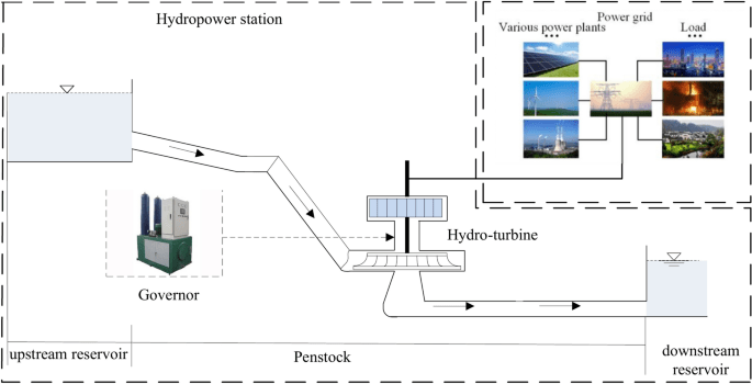
In this investigation, the GCHTGS primarily comprises an upstream reservoir, penstock, governor, hydro-turbine, generator, downstream reservoir, and PG, as illustrated in Fig. 1. The foundational mathematical equations for all subsystems of the GCHTGS coupling framework are presented below.
Schematic representation of GCHTGS.
Prior Penstock Models
Penstock is a crucial element of GCHTGS. The actuation of the guide vanes within the pressure penstock leads to a sudden alteration in flow. Considering the inertia and compressibility of the water mass, the water head in the penstock will fluctuate intensely and periodically.
Factoring in the water elasticity and head loss, the transcendental function of the elongated penstock is expressed as follows
$$G_{P0} (s) = – frac{{T_{w} }}{{T_{e} }}tanh left( {T_{e} s + f} right)$$
(1)
From Eq. (1), it is evident that the mathematical representation of the penstock system is a hyperbolic tangent function, which is not amenable to theoretical stability analysis. Thus, Eq. (1) is expanded via the Taylor series:
$$tanh (x) = frac{sh(x)}{{ch(x)}} = frac{{x + frac{1}{3!}x^{3} + cdot cdot cdot cdot cdot cdot }}{{1 + frac{1}{2!}x^{2} + frac{1}{4!}x^{4} + cdot cdot cdot cdot cdot cdot }}$$
(2)
Various order transfer function models can be derived. The first-order RWHM is frequently applied when the penstock length is short:
$$G_{P1} (s) = – T_{w} s – frac{{T_{w} }}{{T_{e} }}f$$
(3)
When the GCHTGS has an extensive penstock, a more precise model is necessary to elucidate the water hammer phenomenon. Hence, the second-order EWHM and fourth-order EWHM are considered as follows:
$$G_{P2} (s) = – frac{{T_{w} }}{{T_{e} }}frac{{f + T_{e} s}}{{1 + fT_{e} s + frac{1}{2}T_{e}^{2} s^{2} }}$$
(4)
$$G_{P3} (s) = – frac{{T_{w} }}{{T_{e} }}frac{{f + T_{e} s + frac{1}{2}fT_{e}^{2} s^{2} + frac{1}{6}T_{e}^{3} s^{3} }}{{1 + fT_{e} s + frac{1}{2}T_{e}^{2} s^{2} + frac{1}{6}fT_{e}^{3} s^{3} + frac{1}{24}T_{e}^{4} s^{4} }}$$
(5)
Parameter-Varying Penstock Model
It is noticeable that the model’s precision enhances with an increase in order, but excessive order can elevate the computational complexity, as well as induce oscillatory distortions in the time-domain response36. Liu et al.36 introduced a reduced-order EWHM as depicted in Eq. (1).
$$left{ begin{gathered} G_{P4} (s) = – frac{{T_{w} }}{{T_{e} }}frac{{(frac{{2fT_{e}^{2} }}{{pi^{2} }}s^{2} + T_{e} s + f)w_{n}^{2} }}{{s^{2} + 2xi w_{n} s + w_{n}^{2} }} hfill xi { = }frac{{{text{e}}^{f} – {text{e}}^{ – f} }}{{2({text{e}}^{f} {text{ + e}}^{ – f} )}}sqrt {f^{2} + frac{{pi^{2} }}{4}} hfill w_{n} = frac{pi }{{2T_{e} }} hfill end{gathered} right.$$
(6)
In contrast to the second-order EWHM, it accurately conveys the frequency domain resonance peak and extends the effective approximation range from 1 rad/s to 2 rad/s. Concurrently, it circumvents the issue of time-domain oscillatory distortion associated with the fourth-order EWHM, thus more aptly characterizing the water hammer effect in the pressure pipeline. A comparison of the frequency-domain traits of Eq. (1) and Eq. (6) reveals that the reduced-order EWHM demonstrates greater accuracy when the water elasticity coefficient Te is minimal. Conversely, a significant error becomes inevitable with larger Te, as displayed in Fig. 2. The discrepancy between Eq. (1) and Eq. (6) grows with an increase in Te.
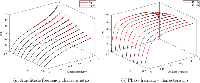
Frequency-domain characteristics at varying values of Te.
Consequently, we introduce a PVM as follows:
$$G_{P5} (s) = – frac{{T_{w} }}{{T_{e} }}frac{{(frac{{2fT_{e}^{2} }}{{pi^{2} }}s^{2} + T_{e} s + f)w_{n}^{2} }}{{sigma s^{2} + 2xi w_{n} s + w_{n}^{2} }}$$
(7)
In Ref.36, the parameter (sigma) was defined as a constant, determined by equating the frequencies of the poles from both the simplified and original models (w_{T} (w_{T} = pi /2T_{e} )). Therefore, model Eq. (6) achieves greater precision at (w_{T}), yet the maximum response frequency ws typically falls short of (omega_{T}) during standard operational conditions for GCHTGS32. Thus, the approach to determining the parameter (sigma) needs to be outlined.
The amplitude and frequency attributes of the transfer functions Eq. (1) and Eq. (7) can be derived by substituting s = jw:
$$G_{P0} (jw) = – frac{{T_{w} }}{{T_{e} }}frac{{1 – e^{ – 2f} e^{{ – j2T_{e} w}} }}{{1 + e^{ – 2f} e^{{ – j2T_{e} w}} }} = – frac{{T_{w} }}{{T_{e} }}frac{{1 – e^{ – 2f} cos (2T_{e} w) + je^{ – 2f} sin (2T_{e} w)}}{{1 + e^{ – 2f} cos (2T_{e} w) – je^{ – 2f} sin (2T_{e} w)}}$$
(8)
$$G_{P5} (jw) = – frac{{T_{w} }}{{T_{e} }}frac{{( – frac{{2fT_{e}^{2} }}{{pi^{2} }}w^{2} + jT_{e} w + f)w_{n}^{2} }}{{ – sigma w^{2} + j2xi w_{n} w + w_{n}^{2} }}$$
(9)
To find an appropriate (sigma), an error function between Eq. (8) and Eq. (9) is formulated as follows:
$$E = sumlimits_{k = 1}^{N} {(left| {G_{P0} (jw_{k} )} right| – left| {G_{P5} (jw_{k} )} right|)^{2} }$$
(10)
where (w_{k}) represents an angular frequency domain ([0,w_{s} ]). The (sigma) can be determined by minimizing the objective.
function founded upon the Grey Wolf Optimizer (GWO) algorithm37, the computation procedures are illustrated in Fig. 3.
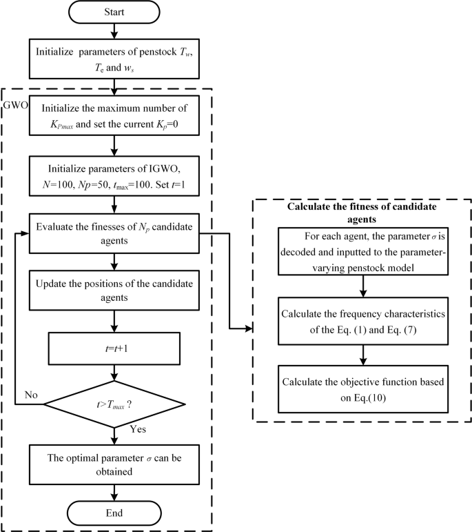
Flow diagram of the computation procedures of (sigma).
Selecting Tw = 2, Te = 1 and f = 0.05, under varying values of ws, the values of the parameter (sigma) are computed and presented in Table 1. The discrepancies between Eq. (6) and Eq. (1), Eq. (7) and Eq. (1) are displayed in Table 2. From Table 1, it can be observed that the parameter (sigma) fluctuates with ws, hence Eq. (7) is referred to as a parameter-varying model (PVM), in which various hydropower plants exhibit distinct values of (sigma). As indicated in Table 1, with the increase of ws, the error rises. Compared to the reduced-order EWHM, the suggested PVM exhibits lesser errors across different ws. Therefore, the proposed PVM achieves superior precision.
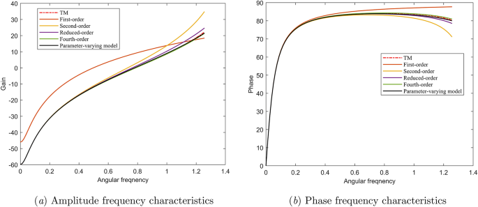
Frequency-domain characteristics under varied penstock models.
Governor
The traditional PI controller is employed for the GCHTGS in this study, defined as follows:
$$G_{PI} (s) = K_{P} + frac{{K_{I} }}{s}$$
(11)
Hydro-turbine
NN model of the hydro-turbine
A precise analytical mathematical model of the hydro-turbine has yet to be established due to its intricate properties. Its dynamic characteristics are generally expressed as38:
$$left{ begin{gathered} M_{t} = M_{t} (y,x_{t} ,H) hfill Q_{t} = Q_{t} (y,x_{t} ,H) hfill end{gathered} right.$$
(12)
The nonlinear hydro-turbine model outlined in Eq. (12) can be linearized via Taylor series expansion for minor disturbances around a steady-state operating point. Equation (12) can be reformulated as39:
$$left{ begin{gathered} m_{t} = e_{y} y + e_{x} x_{t} + e_{h} h hfill q_{t} = e_{qy} y + e_{qx} x_{t} + e_{qh} h hfill end{gathered} right.$$
(13)
where (e_{h} = {{partial m_{t} } mathord{left/ {vphantom {{partial m_{t} } {partial h}}} right. kern-0pt} {partial h}}), (e_{x} = {{partial m_{t} } mathord{left/ {vphantom {{partial m_{t} } {partial x}}} right. kern-0pt} {partial x}}_{t}), (e_{y} = {{partial m_{t} } mathord{left/ {vphantom {{partial m_{t} } {partial y}}} right. kern-0pt} {partial y}}), (e_{qh} = {{partial q_{t} } mathord{left/ {vphantom {{partial q_{t} } {partial h}}} right. kern-0pt} {partial h}}), (e_{qx} = {{partial q_{t} } mathord{left/ {vphantom {{partial q_{t} } {partial x}}} right. kern-0pt} {partial x}}_{t}), (e_{qy} = {{partial q_{t} } mathord{left/ {vphantom {{partial q_{t} } {partial y}}} right. kern-0pt} {partial y}}), the transfer coefficients of torque and discharge, respectively;
The six-coefficient model of the hydro-turbine exemplifies a linearized model under particular operating conditions (determined by water head and GVO). Empirical results based on the linear model are imprecise and cannot be applied to alternate operating conditions. Thus, the six coefficients under various operating circumstances must be established to evaluate stability under FOC. A specific actual measured dataset of the hydro-turbine is depicted in Fig. 5. Nevertheless, the measured data of the hydro-turbine is insufficient, especially for minor openings and low head conditions.
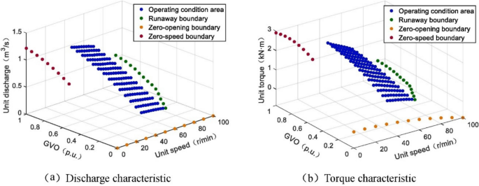
Test data for hydro-turbine.
NN have exceptional nonlinear modeling competency and adaptability. They are capable of learning and capturing intricate patterns and relationships in data, showcasing remarkable generalization ability for forecasting tasks involving unknown situations and new samples. As a result, they have been extensively employed across diverse sectors. In this study, considering the strong nonlinearity and the lacking data of the hydro-turbine, the BPNN is utilized to fit the torque and discharge data. The BPNN training procedure and hydro-turbine BPNN models are depicted in Fig. 6 and Fig. 7, respectively. Figure 7 illustrates that the GVO lines are effectively extended and refined.
Fig. 6
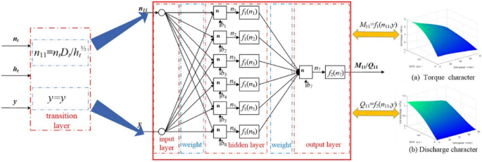
The learning process of BPNN.
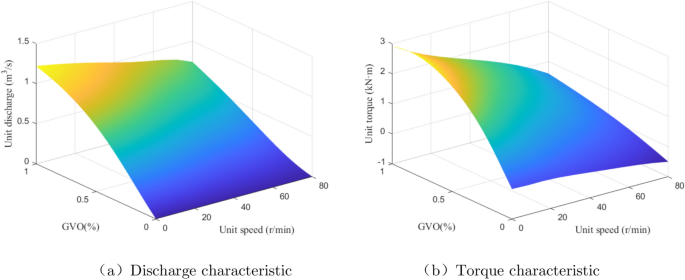
BPNN configurations of Hydro-turbine.
Computation of transfer coefficients for hydro-turbine
A unique method based on the NND is introduced by Liu et al.40 to identify the six transfer coefficients of hydro-turbines. The procedure for this method is outlined below.
(1) Flow rate and torque can be deduced from the BPNN configurations:
$$left{ begin{gathered} Q = f_{Q} left( {n_{11} ,Y} right)D^{2} sqrt H hfill M_{t} = f_{M} left( {n_{11} ,Y} right)D^{3} H hfill end{gathered} right.$$
(14)
(2) Equation (14) can be reformulated as follows:
$$left{ begin{gathered} Q = f_{q2} left( {w_{q2} cdot f_{q1} left( {w_{q1} I + b_{q1} } right) + b_{q2} } right)D^{2} sqrt H n hfill M_{t} = f_{m2} left( {w_{m2} cdot f_{m1} left( {w_{m1} I + b_{m1} } right) + b_{m2} } right)D^{3} Hn hfill end{gathered} right.$$
(15)
In this context, (w_{q1} (w_{m1} )) and (w_{q2} (w_{m2} )) denote the weights of the hidden layer and output layer of the neural network, respectively. (f_{q1} (f_{m1} )) and (f_{q2} (f_{m2} )) represent the activation functions applied in the hidden layer and output layer of the neural network, respectively. (b_{q1} (b_{m1} )) and (b_{q2} (b_{m2} )) illustrate the thresholds for the hidden layer and output layer of the neural network, respectively; (I = left( {n_{11} ,Y} right)) signifies the input for the neural network.
(3) By taking the partial derivatives of the prior functional relationship, we derive the general expression for the transfer coefficients.
$$left{ begin{gathered} e_{qy} = frac{{Y_{m} }}{{Q_{r} }}frac{partial Q}{{partial Y}} = frac{{Y_{m} }}{{Q_{r} }}D^{2} sqrt H f_{q2}^{prime } w_{q2} f_{q1}^{prime } w_{q1} frac{partial I}{{partial Y}} hfill e_{qh} = frac{{H_{r} }}{{Q_{r} }}frac{partial Q}{{partial H}} = frac{{H_{r} }}{{Q_{r} }}left( {frac{{D^{2} }}{2sqrt H }f_{Q} + D^{2} sqrt H f_{q2}^{prime } w_{q2} f_{q1}^{prime } w_{q1} frac{partial I}{{partial H}}} right) hfill e_{qx} = frac{{X_{r} }}{{Q_{r} }}frac{partial Q}{{partial X}} = frac{{X_{r} }}{{Q_{r} }}D^{2} sqrt H f_{q2}^{prime } w_{q2} f_{q1}^{prime } w_{q1} frac{partial I}{{partial X}} hfill e_{y} = frac{{Y_{m} }}{{M_{r} }}frac{{partial M_{t} }}{partial Y} = frac{{Y_{m} }}{{M_{r} }}D^{3} Hf_{m2}^{prime } w_{m2} f_{m1}^{prime } w_{m1} frac{partial I}{{partial Y}} hfill e_{h} = frac{{H_{r} }}{{M_{r} }}frac{{partial M_{t} }}{partial H} = frac{{H_{r} }}{{M_{r} }}left( {D^{3} f_{M} + D^{3} Hf_{m2}^{prime } w_{m2} f_{m1}^{prime } w_{m1} frac{partial I}{{partial H}}} right) hfill e_{x} = frac{{X_{r} }}{{M_{r} }}frac{{partial M_{t} }}{partial X} = frac{{X_{r} }}{{M_{r} }}D^{3} Hf_{m2}^{prime } w_{m2} f_{m1}^{prime } w_{m1} frac{partial I}{{partial X}} hfill end{gathered} right.$$
(16)
Generator and Load
For the GCHTGS, a second-order synchronous generator framework is utilized, with its differential equations illustrated41:
$$left{ begin{gathered} T_{a} frac{{dx_{t} }}{dt} = m_{t} – left( {e_{g} x_{t} + K_{a} xi_{1} + D_{a} left( {x_{t} – x_{s} } right) + m_{g} } right) hfill frac{{dxi_{1} }}{dt} = x_{t} – x_{s} hfill end{gathered} right.$$
(17)
Power grid
To evaluate the stability of the GCHTGS system, establishing a straightforward PG mathematical model that can express the load and frequency traits is essential. In this work, the PG is conceptualized as an equivalent generator, and its linear model can be derived. The comprehensive framework of the simplified PG is depicted in Fig. 8. If the disturbance of the PG load is disregarded, i.e., (Delta p_{g} = 0), the fundamental equation of the power grid is:
$$left{ begin{gathered} frac{{dx_{s} }}{dt} = frac{1}{{T_{s} }}left( {Bp_{t} – D_{s} x_{s} – frac{1}{{T_{g} R_{g} }}xi_{2} } right) hfill frac{{dxi_{2} }}{dt} = x_{s} – frac{1}{{T_{g} }}xi_{2} hfill end{gathered} right.$$
(18)
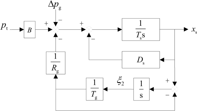
Block diagram of the equivalent PG.
By merging Eq. (7), Eq. (11), Eq. (13), and Eq. (17)-(18), the state equation of GCHTGS considering the proposed PVM can be formulated as Eq. (19). It should be acknowledged that r1 and r2 are the intermediate state variables. In a similar fashion, the state equations of GCHTGS incorporating first-order RWHM, second-order EWHM, and fourth-order EWHM are documented as Eq. (20)-(22).
$$left{ begin{gathered} dot{x}_{t} = frac{1}{{T_{a} }}left[ {e_{y} y + (e_{x} – e_{g} – D_{a} )x_{t} + e_{h} h – K_{a} xi_{1} + D_{a} x_{s} – m_{g} } right] hfill dot{y} = – left[ {frac{{K_{P} }}{{T_{a} }}left( {e_{x} – e_{g} – D_{a} } right) + K_{I} } right]x_{t} – frac{{K_{P} }}{{T_{a} }}left[ {e_{y} y + e_{h} h – K_{a} xi_{1} + D_{a} x_{s} – m_{g} } right] hfill dot{x}_{s} = frac{1}{{T_{s} }}left[ {D_{a} Bx_{t} – left( {D_{s} + D_{a} B} right)x_{s} + K_{a} Bxi_{1} – frac{1}{{R_{g} T_{g} }}xi_{2} } right] hfill dot{xi }_{1} = x_{t} – x_{s} hfill dot{xi }_{2} = x_{s} – frac{1}{{T_{g} }}xi_{2} hfill dot{r}_{1} = r_{2} hfill dot{r}_{2} = frac{{ – 2xi w_{n} }}{alpha }r_{2} – frac{{w_{n}^{2} }}{alpha }r_{1} + e_{qx} x_{t} + e_{qy} y + e_{qh} h hfill h = – frac{{T_{w} fw_{n}^{2} }}{{T_{e} alpha }}r_{1} – frac{{T_{w} w_{n}^{2} }}{alpha }r_{2} hfill end{gathered} right.$$
(19)
$$left{ begin{gathered} dot{x}_{t} = frac{1}{{T_{a} }}left[ {e_{y} y + (e_{x} – e_{g} – D_{a} )x_{t} + e_{h} h – K_{a} xi_{1}
+ D_{a} x_{s} – m_{g} } right] hfill dot{y} = – left[ {frac{{K_{P} }}{{T_{a} }}left( {e_{x} – e_{g} – D_{a} } right) + K_{I} } right]x_{t} – frac{{K_{P} }}{{T_{a} }}left[ {e_{y} y + e_{h} h – K_{a} xi_{1} + D_{a} x_{s} – m_{g} } right] hfill dot{x}_{s} = frac{1}{{T_{s} }}left[ {D_{a} Bx_{t} – left( {D_{s} + D_{a} B} right)x_{s} + K_{a} Bxi_{1} – frac{1}{{R_{g} T_{g} }}xi_{2} } right] hfill dot{xi }_{1} = x_{t} – x_{s} hfill dot{xi }_{2} = x_{s} – frac{1}{{T_{g} }}xi_{2} hfill dot{h} = x_{t} left( {frac{{e_{qx} – e_{qy} K_{p} }}{{T_{a} e_{qh} }}D_{a} + frac{{e_{qy} K_{p} – e_{qx} }}{{T_{a} e_{qh} }}(e_{x} – e_{g} ) + frac{{K_{i} e_{qy} }}{{e_{qh} }}{ + }frac{{fe_{qx} T_{w} }}{{e_{qh} T_{e} }}} right) hfill + x_{s} left( {frac{{e_{qy} K_{p} – e_{qx} }}{{T_{a} e_{qh} }}D_{a} } right) + xi_{1} left( {frac{{K_{a} e_{qx} }}{{T_{a} e_{qh} }} – frac{{K_{a} e_{qy} K_{p} }}{{T_{a} e_{qh} }}} right) + frac{{e_{qx} – e_{qy} K_{p} }}{{T_{a} e_{qh} }}m_{g} hfill + hleft( {frac{{e_{qy} K_{p} – e_{qx} }}{{T_{a} e_{qh} }}e_{h} – frac{1}{{e_{qh} T_{w} }} + frac{{fT_{w} }}{{T_{e} }}} right) + yleft( {frac{{e_{qy} K_{p} – e_{qx} }}{{T_{a} e_{qh} }}e_{y} + frac{{fe_{qy} T_{w} }}{{e_{qh} T_{e} }}} right) hfill end{gathered} right.$$
(20)
$$left{ begin{gathered} dot{x}_{t} = frac{1}{{T_{a} }}left[ {e_{y} y + (e_{x} – e_{g} – D_{a} )x_{t} – frac{{2T_{w} }}{{T_{e}^{2} }}r_{2} e_{h} – K_{a} xi_{1} + D_{a} x_{s} – m_{g} } right] hfill dot{y} = – left[ {frac{{K_{P} }}{{T_{a} }}left( {e_{x} – e_{g} – D_{a} } right) + K_{I} } right]x_{t} – frac{{K_{P} }}{{T_{a} }}left[ {e_{y} y – frac{{2T_{w} }}{{T_{e}^{2} }}r_{2} e_{h} – K_{a} xi_{1} + D_{a} x_{s} – m_{g} } right] hfill dot{x}_{s} = frac{1}{{T_{s} }}left[ {D_{a} Bx_{t} – left( {D_{s} + D_{a} B} right)x_{s} + K_{a} Bxi_{1} – frac{1}{{R_{g} T_{g} }}xi_{2} } right] hfill dot{xi }_{1} = x_{t} – x_{s} hfill dot{xi }_{2} = x_{s} – frac{1}{{T_{g} }}xi_{2} hfill dot{r}_{1} = r_{2} hfill dot{r}_{2} = – frac{2}{{T_{e}^{2} }}r_{1} – frac{2f}{{T_{e} }}r_{2} + e_{qx} x_{t} + e_{qy} y + e_{qh} h hfill h = – frac{{2fT_{w} }}{{T_{e}^{3} }}r_{1} – frac{{2T_{w} }}{{T_{e}^{2} }}r_{2} hfill end{gathered} right.$$
(21)
$$left{ begin{gathered} dot{x}_{t} = frac{1}{{T_{a} }}left[ {e_{y} y + (e_{x} – e_{g} – D_{a} )x_{t} + e_{h} h – K_{a} xi_{1} + D_{a} x_{s} – m_{g} } right] hfill dot{y} = – left[ {frac{{K_{P} }}{{T_{a} }}left( {e_{x} – e_{g} – D_{a} } right) + K_{I} } right]x_{t} – frac{{K_{P} }}{{T_{a} }}left[ {e_{y} y + e_{h} h – K_{a} xi_{1} + D_{a} x_{s} – m_{g} } right] hfill dot{x}_{s} = frac{1}{{T_{s} }}left[ {D_{a} Bx_{t} – left( {D_{s} + D_{a} B} right)x_{s} + K_{a} Bxi_{1} – frac{1}{{R_{g} T_{g} }}xi_{2} } right] hfill dot{xi }_{1} = x_{t} – x_{s} hfill dot{xi }_{2} = x_{s} – frac{1}{{T_{g} }}xi_{2} hfill dot{r}_{1} = r_{2} hfill dot{r}_{2} = r_{3} hfill dot{r}_{3} = r_{4} hfill dot{r}_{4} = – frac{24}{{T_{e}^{4} }}r_{1} – frac{24f}{{T_{e}^{3} }}r_{2} – frac{12}{{T_{e}^{2} }}r_{3} – frac{4f}{{T_{e} }}r_{4} + e_{qx} x_{t} + e_{qy} y + e_{qh} h hfill h = – frac{{24fT_{w} }}{{T_{e}^{5} }}r_{1} – frac{{24T_{w} }}{{T_{e}^{4} }}r_{2} – frac{{12fT_{w} }}{{T_{e}^{3} }}r_{3} – frac{{4T_{w} }}{{T_{e}^{2} }}r_{4} hfill end{gathered} right.$$
(22)
Verification of the model
Subsequent to being linked to the grid, hydroelectric systems can utilize wicket gate adjustment mode, power adjustment mode, or frequency adjustment mode. The application of frequency adjustment mode by hydroelectric systems under grid-connected circumstances can not only effectively manage grid frequency variances and guarantee the secure and consistent operation of the power network but also serve a crucial regulatory function in the context of extensive integration of new energy sources. Hence, frequency adjustment mode is also a significant regulation mode for systems post grid connection. This document primarily considers frequency adjustment mode as a case study to examine the effects of distinct pipeline models and operating conditions on the stability of the systems. In upcoming investigations, we will delve deeper into the stability under alternative regulation modes, such as power adjustment mode.
To validate the accuracy and efficacy of the proposed model delineated by Eq. (19), the dynamic response process (DRP) of the models expressed by Eq. (19)-(22) are contrasted with those of the GCHTGS considering the transcendental model of the penstock system. For the GCHTGS system, the load disturbance serves as the external disturbance. The parameters’ values and the simulation block diagram of the GCHTGS system are illustrated in Table 3 and Fig. 9.
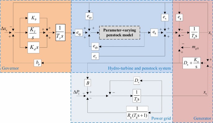
Block diagram of the GCHTGS.
The results of the DRP of the GCHTGS system considering various penstock models are depicted in Fig. 10(a). Additionally, the deviation of distinct penstock models relative to TM is presented in Fig. 10(b). From Fig. 10, the DRP of the rotational speed of the GCHTGS system when accounting for the fourth-order EWHM, PVM, and TM models are nearly identical. The findings indicate that the PVM and fourth-order EWHM exhibit greater precision. The DRP of the second-order EWHM and the reduced-order EWHM displays minor discrepancies from TM, particularly in the peaks and troughs areas. Nevertheless, the DRP of the first-order RWHM shows considerable divergence from TM. It is distinctly evident that the DRP of the first-order RWHM has a different oscillation period compared to the second-order EWHM, reduced-order EWHM, fourth-order EWHM, PVM, and TM. The accuracy and efficiency of the proposed PVM for the GCHTGS system have been confirmed.
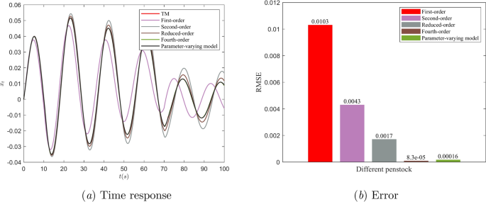
Comparison of various penstock models, (a) Time response, (b) Error.

