
Regulating formulas and also service
The circumstance thought about in the research is the wave communication with a gadget created as a row of plates, which can relocate flat in piston-type oscillations. Home plates are linked by flexible-type joinings. The circumstance is revealed schematically in Fig. 1, where χ ( y, z, t) is home plate variation.
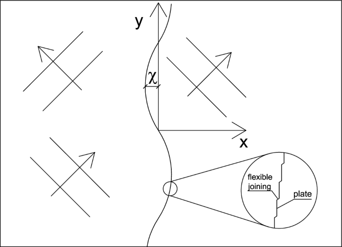
Lay out of the serpent-type wave power converter with the coordinate system.
The service for the wave-device communications is obtained on the basis of the prospective wave concept, which is a conventional concept made use of in the modelling of wave power converters. This strategy has some restrictions and also calls for the adhering to presumptions. The liquid is incompressible and also inviscid, and also the liquid activity is irrotational. It is presumed that the sea base is invulnerable, and also that the excitation is given by occurrence waves of little amplitude
A and also regularity ω. These are sensible and also extensively identified estimations used in the evaluations of actual functioning WECs. According to these presumptions, the rate vector, V ( x, y, z, t), might be calculated from the rate prospective Φ (
x, y, z, t
)
$$ {varvec {V}} =mathrm {Delta Phi} ( x, y, z, tright),$$
( 1 ).
where ∇
(
) is the two-dimensional vector differential driver
The liquid activity is regulated by the connection formula
$$ {nabla} ^ {2} Phi =0,$$
( 2 ).
The kinematic border problem,
$$ {upeta} _ {mathrm {t}} + {Phi} _ {x} {upeta} _ {mathrm {x}} + {Phi} _ {mathrm {y}} {upeta} _ {mathrm {y}} – {Phi} _ {mathrm {z}} =0, z= upeta left( x, y, tright).$$
( 3 ).
The vibrant border problem,
$$ {Phi} _ {mathrm {t}} +gupeta +frac {1} {2} nablaPhi ^ {2} =0, z= upeta left( x, y, tright).$$
( 4 ).
The kinematic border at the wave power converter,
$$ {upchi} _ {mathrm {t}} + {Phi} _ {mathrm {y}} {upchi} _ {mathrm {y}} + {Phi} _ {mathrm {z}} {upchi} _ {mathrm {z}} – {Phi} _ {mathrm {x}} =0, x =upchi left( y, z, tright),$$
( 5 ).
and also at the sea base, the adhering to border problem have to be pleased,$$ {Phi} _ {mathrm {z}} = 0, z = -h,$$
( 6 ).
where η ( x, y, t) is the complimentary surface area oscillation, g= 9.81 m/s 2
is the velocity because of gravity, and also h is the water deepness.
Additionally, the rate possibility have to please the border problems at infinity and also preliminary problems 27,28 To get a logical service of the boundary-value issue and also to stay clear of troubles developing from an unidentified place of the complimentary surface area η ( x, y, t),
the Taylor collection development strategy and also the perturbation approach are used. The free-surface kinematic and also vibrant border problems and also the kinematic border problem at the wave power converter were increased right into Taylor collection concerning a mean setting
29
$$ amount _ {n= 0} ^ {infty} frac {{upeta} ^ {n}} {n!} frac {{partial} ^ {n}} {partial {z} ^ {n}} ({upeta} _ {mathrm {t}} + {Phi} _ {mathrm {x}} {upeta} _ {mathrm {x}} + {Phi} _ {mathrm {y}} {upeta} _ {mathrm {y}} – {Phi} _ {mathrm {z}} )= 0, z= 0,$$
( 7 ).
$$ amount _ {n= 0} ^ {infty} frac {{upeta} ^ {n}} {n!} frac {{partial} ^ {n}} {partial {z} ^ {n}} ({Phi} _ {mathrm {t}} +gupeta +frac {1} {2} ^ {2} )= 0, z= 0$$
( 8 ).
$$ amount _ {n= 0} ^ {infty} frac {{upchi} ^ {n}} {n!} frac {{partial} ^ {n}} {partial {x} ^ {n}} ({upchi} _ {mathrm {t}} + {Phi} _ {mathrm {y}} {upchi} _ {mathrm {y}} + {Phi} _ {mathrm {z}} {upchi} _ {mathrm {z}} – {Phi} _ {mathrm {x}} )= 0, x= 0$$
( 9 ).
The application of Eq. ( 2) to (1) leads to adhering to
$$ {nabla} ^ {2} Phi =0,$$
( 10 ).
$$ {Phi} _ {mathrm {t}} +gupeta +frac {1} {2} nablaPhi ^ {2} =0, z= 0,$$
( 11 ).
$$ {upeta} _ {mathrm {t}} – {Phi} _ {z} -upeta {Phi} _ {zz} + {Phi} _ {mathrm {x}} {upeta} _ {mathrm {x}} + {Phi} _ {mathrm {y}} {upeta} _ {mathrm {y}} =0, z= 0$$
( 12 ).
$$ {upchi} _ {mathrm {t}} + {Phi} _ {mathrm {y}} {upchi} _ {mathrm {y}} + {Phi} _ {mathrm {z}} {upchi} _ {mathrm {z}} – {Phi} _ {mathrm {x}} – {mathrm {chi Phi}} _ {mathrm {xx}} =0, x =0$$
( 13 ).
$$ {Phi} _ {mathrm {z}} =0, z=- mathrm {h} $$
( 14 ).
By presuming perturbation treatment
$$ Phi = {} _ {1} Phi + {} _ {2} Phi + …,$$
( 15 ).
$$ upeta = {} _ {1} upeta + {} _ {2} upeta + …,$$
( 16 ).
where an amount with a left n, n= 0, 1, … is of order of ( Ak) n in which A is the particular wave amplitude, k
is the particular wave number and also
Ak
= ε ≤ 1.[phi {mathrm{e}}^{-iupomega t}right] All the list below evaluation will certainly relate to the initial order service of the perturbation approach and also for the function of quality, the left will certainly be overlooked.
To additionally damage down the service, the spatial rate possibility is presented, such that
$$ Phi =mathrm {Re}
,$$
( 17 ).
where ϕ( x, y, z) is the spatial rate possibility. The occurrence ϕ I
, mirrored ϕ
1
and also transferred ϕ
2
spatial rate possibilities might be composed in the list below type
$$ {phi} _ {I} =frac {-igA} {upomega} frac {mathrm {cos} {alpha} _ {1} {left( z+ hright)} |( z+ hright)}} {mathrm {cos} {mathrm {alpha}} _ {1} h} mathrm {exp} {left(- {|(- {} mathrm {alpha}} _ {1} mathrm {costheta} x- {mathrm {alpha}} _ {1} sinuptheta yright),$$
( 18 ).
$$ {phi} _ {1} = {phi} _ {I} +amount _ {j= 1} frac {-ig {R} _ {j}} {upomega} frac {mathrm {cos} {alpha} _ {j} {left( z+ hright)} |( z+ hright)}} {mathrm {cos} {mathrm {alpha}} _ {mathrm {j}} h} mathrm {exp} {left(- {|(- {} upbeta} _ {mathrm {j}} x- {mathrm {alpha}} _ {1} sinuptheta yright),$$
( 19 ).
$$ {phi} _ {2} =amount _ {j= 1} frac {-ig {T} _ {j}} {upomega} frac {mathrm {cos} {alpha} _ {j} {left( z+ hright)} |( z+ hright)}} {mathrm {cos} {mathrm {alpha}} _ {mathrm {j}} h} mathrm {exp} {left(- {|(- {} upbeta} _ {mathrm {j}} x- {mathrm {alpha}} _ {1} sinuptheta yright),$$
( 20 ).
offered that$$ frac {{omega} ^ {2}} {g} =- {mathrm {alpha}} _ {mathrm {j}} mathrm {tan} {mathrm {alpha}} _ {mathrm {j}} h, jge 1$$
( 21 ).
$$ {upbeta} _ {mathrm {j}} =sqrt {{mathrm {alpha}} _ {mathrm {j}} ^ {2} – {mathrm {alpha}} _ {1} ^ {2} {mathrm {wrong}} ^ {2} uptheta},$$
( 22 ).
where θ is the wave breeding angle and also the eigenvalues are: α j= {– ik, α 2
, α 3, …}, where k is the wavenumber. The coefficients R j can be obtained by increasing the wave power converter’s kinematic border problem (13) by orthogonal features, cos α j= {cos α 1, cos α
2
, …}, and afterwards incorporating the item, to ensure that the service for every
R
j
is$$ {upchi} _ {10} {mathrm {wrong}} ^ {2} {mathrm {alpha}} _ {mathrm {j}} h= {updelta} _ {1mathrm {j}} {} _ {1} {mathrm {alpha}} _ {1} mathrm {costheta} frac {2 {mathrm {alpha}} _ {1} h+ mathrm {wrong} 2 {mathrm {alpha}} _ {1} h} {4 {mathrm {alpha}} _ {1}} – {upbeta} _ {mathrm {j}} {R} _ {j} frac {2 {mathrm {alpha}} _ {mathrm {j}} h+ mathrm {wrong} 2 {mathrm {alpha}} _ {mathrm {j}} h} {4 {mathrm {alpha}} _ {mathrm {j}}},$$
( 23 ).
$$ {{R} _ {j} =updelta} _ {1mathrm {j}} {} _ {1} {mathrm {alpha}} _ {1} frac {mathrm {costheta}} {{upbeta} _ {1}} -4 {upchi} _ {10} {mathrm {alpha}} _ {mathrm {j}} frac {{mathrm {wrong}} ^ {2} {mathrm {alpha}} _ {mathrm {j}} h} {{upbeta} _ {mathrm {j}} {left( 2 {|( 2 {} mathrm {alpha}} _ {mathrm {j}} h+ mathrm {wrong} 2 {mathrm {alpha}} _ {mathrm {j}} hright)},$$
( 24 ).
A comparable treatment is put on get the coefficients
T
j
$$ iupomega {upchi} _ {10} =- frac {ig} {upomega} amount {upbeta} _ {mathrm {j}} {T} _ {j} frac {mathrm {cos} {mathrm {alpha}} _ {mathrm {j}} {left( z+ hright)} |( z+ hright)}} {mathrm {cos} {mathrm {alpha}} _ {mathrm {j}} h},$$
( 25 ).
$$ {upchi} _ {10} {wrong} ^ {2} {mathrm {alpha}} _ {mathrm {j}} h= {upbeta} _ {mathrm {j}} {T} _ {j} frac {2 {mathrm {alpha}} _ {mathrm {j}} h+ mathrm {wrong} 2 {mathrm {alpha}} _ {mathrm {j}} h} {4 {mathrm {alpha}} _ {mathrm {j}}},$$
( 26 ).
$$ {T} _ {j} =frac {{4upchi} _ {10} {{mathrm {alpha}} _ {mathrm {j}} wrong} ^ {2} {mathrm {alpha}} _ {mathrm {j}} h} {{upbeta} _ {mathrm {j}} {left( 2 {|( 2 {} mathrm {alpha}} _ {mathrm {j}} h+ mathrm {wrong} 2 {mathrm {alpha}} _ {mathrm {j}} hright)},$$
( 27 ).
where$$ {upchi} _ {1} = {upchi} _ {10} {mathrm {e}} ^ {-iupomega t}.$$
( 28 ).
The generalised hydrodynamic pressures ( F)
for a row of wave power converters can be determined at a provided place by incorporating the wave stress
p
that is acting upon the wave power converter. As necessary, where
n
is the generalised regular vector.
$$ {varvec {F}} = {int} _ {-h} ^ {0} p {varvec {n}} dz,$$
( 29 ).
$$ p= imathrm {omega rho} phi {mathrm {e}} ^ {-iupomega t}.$$
( 30 ).
The complex-valued amplitude of a straight pressure is
$$ {F} _ {10} =uprho gleft( Afrac {mathrm {tan} {mathrm {alpha}} _ {1} h} {{mathrm {alpha}} _ {1}} +amount _ {j= 1} {mathrm {R}} _ {mathrm {j}} frac {mathrm {tan} {mathrm {alpha}} _ {j} h} {{mathrm {alpha}} _ {j}} -amount _ {j= 1} {mathrm {T}} _ {mathrm {j}} frac {mathrm {tan} {mathrm {alpha}} _ {j} h} {{mathrm {alpha}} _ {j}} )$$
( 31 ).
Analogously, the spatial energy influencing the converter relative to the sea base
( 31 ).
Analogously, the spatial energy influencing the converter relative to the sea base
$$ {F} _ {50} =uprho gleft( Afrac {{mathrm {alpha}} _ {1} hmathrm {wrong} {mathrm {alpha}} _ {1} h+ mathrm {cos} {mathrm {alpha}} _ {1} h-1} {{mathrm {alpha}} _ {1} ^ {2} mathrm {cos} {mathrm {alpha}} _ {1} h} +amount _ {j= 1} {mathrm {R}} _ {mathrm {j}} frac {{mathrm {alpha}} _ {j} hmathrm {wrong} {mathrm {alpha}} _ {j} h+ mathrm {cos} {mathrm {alpha}} _ {j}} {{mathrm {alpha}} _ {j} ^ {2} mathrm {cos} {mathrm {alpha}} _ {j} h} -amount _ {j= 1} {mathrm {T}} _ {mathrm {j}} frac {{mathrm {alpha}} _ {j} hmathrm {wrong} {mathrm {alpha}} _ {j} h+ mathrm {cos} {mathrm {alpha}} _ {j}} {{mathrm {alpha}} _ {j} ^ {2} mathrm {cos} {mathrm {alpha}} _ {j} h} ).$$
( 32 ).
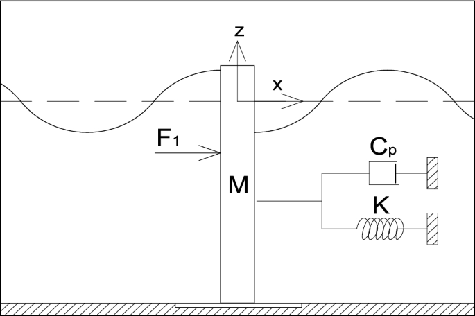
Formula of activity
The 2nd component of the evaluation carries out and also develops to the version the formula of activity defining the results of the hydrodynamic pressure on the activity of the wave power converter (Fig. 2). The formula might be composed in the list below type
$$ M {upchi} _ {1} ^ {{prime} {prime}} + {C} _ {p} {upchi} _ {1} {prime} +K {upchi} _ {1} = {F} _ {1},$$
( 33 ).
which might be composed as Number 2 The schematic sight power liftoff system.$$- M {upomega} ^ {2} {upchi} _ {10} -i {upomega C} _ {p} {upchi} _ {10} +K {upchi} _ {10} = {F} _ {10},$$
( 34 ).
in which M
— the mass of the framework,
C
p
— the power liftoff coefficient and also K— the rigidity coefficient.
By supplying the pressure acquired from the Bernoulli formula, the formula of activity might be composed as adheres to
$$- M {upomega} ^ {2} {upchi} _ {10} -i {upomega C} _ {p} {upchi} _ {10} +K {upchi} _ {10} =uprho gAfrac {mathrm {tan} {mathrm {alpha}} _ {1} h} {{mathrm {alpha}} _ {1}} +uprho gsum _ {j= 1} {mathrm {R}} _ {mathrm {j}} frac {mathrm {tan} {mathrm {alpha}} _ {j} h} {{mathrm {alpha}} _ {j}} -uprho gsum _ {j= 1} {mathrm {T}} _ {mathrm {j}} frac {mathrm {tan} {mathrm {alpha}} _ {j} h} {{mathrm {alpha}} _ {j}},$$
( 35 ).
which after using (24) and also (27) ultimately leads to a formula for χ
10
composed as adheres to$$ {upchi} _ {10} {left(- M {|(- M {} upomega} ^ {2} -i {upomega C} _ {p} +K +8 uprho gsum _ {j= 1} frac {{wrong} ^ {2} {mathrm {alpha}} _ {mathrm {j}} h} {{upbeta} _ {mathrm {j}} {left( 2 {|( 2 {} mathrm {alpha}} _ {mathrm {j}} h+ mathrm {wrong} 2 {mathrm {alpha}} _ {mathrm {j}} hright) cos {mathrm {alpha}} _ {mathrm {j}} h} {right)= 2uprho gAfrac {|)= 2uprho gAfrac {} mathrm {tan} {mathrm {alpha}} _ {1} h} {{mathrm {alpha}} _ {1}}.$$
( 36 ).
The Eq. ( 36) might be composed as adheres to
$$ {upchi} _ {10} {left(- {|(- {} upomega} ^ {2} {left( M+ mu right)+ K-iupomega left( {|( M+ mu right)+ K-iupomega left( {} C} _ {p} +Cright) right)= {F} _ {D10},$$
( 37 ).
in which we specify μ as included mass and also
C as included damping$$ mu =amount _ {j= 1} 8uprho frac {{wrong} ^ {2} {mathrm {alpha}} _ {mathrm {j}} h} {{{mathrm {alpha}} _ {mathrm {j}} upbeta} _ {mathrm {j}} {left( 2 {|( 2 {} mathrm {alpha}} _ {mathrm {j}} h+ mathrm {wrong} 2 {mathrm {alpha}} _ {mathrm {j}} hright)},$$
( 38 ).
$$ C= 8mathrm {rho omega} frac {{wrong} ^ {2} {mathrm {alpha}} _ {1} h} {{{imathrm {alpha}} _ {1} upbeta} _ {1} {left( 2 {|( 2 {} mathrm {alpha}} _ {1} h+ mathrm {wrong} 2 {mathrm {alpha}} _ {1} hright)},$$
( 39 ).
and also F D10 as the pressure because of diffracted waves$$ {F} _ {D10} =2uprho gAfrac {mathrm {tan} {mathrm {alpha}} _ {1} h} {{mathrm {alpha}} _ {1}},$$
( 40 ).
The activity of a wave power converter relies on the worth of the coefficient C p The choice of an ideal C p is a facility issue. For little worths of C p, the wave power emits from a conversion system in the type of mirrored and also transferred waves, and also the performance of a wave power converter is reduced. When the worths of C p are huge, the wave power emit from a system in the type of mirrored waves, and also the performance of a wave power converter is once again reduced. These suggest that there is an ideal worth of
C
p
The ideal worth of C p
might be obtained analytically by establishing the minimum of wave power emitted from a wave power converter
$$ {| {T} _ {1}|} ^ {2} + {| {R} _ {1}|} ^ {2} = {} ^ {2} -4 Aleft( {upchi} _ {10} +overline {{upchi} _ {10}} {right) left( frac {|) left( frac {} {mathrm {sinh}} ^ {2} kh} {2kh+ mathrm {sinh} 2kh} {right) +32 {|) +32 {} upchi} _ {10} overline {{upchi} _ {10}} {{left( frac {|( frac {} {mathrm {sinh}} ^ {2} kh} {2kh+ mathrm {sinh} 2kh} {right)} |)}} ^ {2},$$[{left(K-{upomega }^{2}left(M+mu right)right)}^{2}+{upomega }^{2}{left(C+{C}_{p}right)}^{2}right]
( 41 ).
where [{left(K-{upomega }^{2}left(M+mu right)right)}^{2}+{upomega }^{2}{left(C+{C}_{p}right)}^{2}right]( overline {{chi} _ {10}} )
is the complicated conjugate.
After some algebra one acquires$$ -8 {A F} _ {D10} upomega frac {{upomega} ^ {2} {left(- {|(- {} C} ^ {2} -2 C {C} _ {p} + {{left( M+ mu right)} |( M+ mu right)}} ^ {2} {upomega} ^ {2} – {C} _ {p} ^ {2} {right)+ {|)+ {} K} ^ {2} -2 K {upomega} ^ {2} {left( M+ mu right)} |( M+ mu right)}} {{{left} |
}} ^ {2}} frac {{mathrm {sinh}} ^ {2} kh} {2kh+ mathrm {sinh} 2kh} $$
$$ -64 {{F} _ {D10}} ^ {2} {upomega} ^ {2} frac {C+ {C} _ {p}} {{{left
} |
}} ^ {2}} {{left( frac {|( frac {} {mathrm {sinh}} ^ {2} kh} {2kh+ mathrm {sinh} 2kh} {right)} |)}} ^ {2} =0,$$
( 42 ).
which leads to streamlined sophisticated formula for C p$$ {C} _ {p} =sqrt {{{left( K/upomega -upomega left( M+ mu right) right)} |( K/upomega -upomega left( M+ mu right) right)}} ^ {2} + {C} ^ {2}},$$
( 43 ).
{
since
$$ C= -8 mathrm {| Due to the fact that$$ C= -8 mathrm {,} rho omega} frac {{sinh} ^ {2} kh} {{{mathrm {alpha}} _ {1}} ^ {2} {left( 2kh+ mathrm {|( 2kh+ mathrm {} sinh} 2khright)} =4frac {{F} _ {D10}} {Aupomega} frac {{sinh} ^ {2} kh} {2kh+ mathrm {sinh} 2kh},$$
( 44 ).
For additional assessment of a wave power converter performance, the occurrence wave power
P
I
is determined from
$$ {P} _ {I} =frac {1} {4} frac {uprho g {} ^ {2} upomega} {k} {left( 1+ frac {|( 1+ frac {} 2kh} {mathrm {sinh} 2kh} ),$$(*)
( 45 ).
(*) the power recorded (*) P(*) c(*) by the converter is(*)$$ {P} _ {c} =frac {1} {2} {C} _ {p} {upomega} ^ {2} frac {{ {F} _ {D10} } ^ {2}} {{{left( K- {|( K- {} upomega} ^ {2} {left( M+ mu right) right)} |( M+ mu right) right)}} ^ {2} + {{left( upomega left( C+ {|( upomega left( C+ {} C} _ {p} {right) right)} |) right)}} ^ {2}},$$(*)
( 46 ).
(*) which might be additional streamlined to(*)$$ {P} _ {c} =frac {{ {F} _ {D10} } ^ {2}} {4 {C} _ {p} +4 C}.$$(*)
( 47 ).
(*)