Fatigue damage reduction in hydropower startups with machine learning

Data collection

The first experimental campaign dataset contains measurements of the input and output quantities for about 100 transient operations of a reduced-scale model of Francis turbines for four different startup types. In these tests, strain gauges are attached to both the guide vanes axis and the runner blades to measure the mechanical stresses. Analog signals of the measurements are acquired through a National Instrument (NI) Compact DAQ system and an NI PXI system for pressure fluctuations and stresses. The duration of the time series varied from 7 to 60 seconds with a maximal frequency of measurements of 5000Hz. Some of the observations had different frequencies, which were harmonized during pre-processing by down-sampling all signals to 1000Hz.

The stresses induced in the turbine depend primarily on two control variables: the rotational speed of the runner and the discharge. As the discharge observations suffer from measurement noise, the GVO variable is used, as the characteristic curve of the hydraulic machine bonds the turbine discharge with its guide vane opening passage. In the reduced-scale model platform, a feeding pump attempts to maintain a constant Head during the start-up. In practice, abrupt changes in discharge due to rapid opening of the guide vanes lead to a decrease in Head, which is compensated by a quick increase of the feeding pump speed. Due to the pump’s inability to instantly adjust, Head measurements may fluctuate. Hence, to construct the model of the stresses we use the Head, GVO and turbine speed as the inputs. During the trajectory optimization, we vary only two parameters, the Turbine Speed and the GVO, and keep the Head at a fixed level.

The data consists of real measurements of four sensors positioned with the turbine of the reduced scale model, collected for four different start-up types. We examined each type at different time scales, corresponding to Froude numbers in the range of {0.9, 1.0, 1.2, 2.4, 3.6, 4.8, 6, 7.2}. Trajectories shorter in time correspond to smaller Froude numbers, see Fig. 6. Measurements were collected for inputs (GVO, Turbine speed, Head) and outputs (stresses in several positions in the turbine). Each experiment was repeated ten times. The extreme conditions within the turbine sometimes led to sensor failure, causing uncontrolled drifting or high oscillations and rendering some measurements unusable. The model was trained on all runs that did not show visible drifts or other excessive noise. Out of four sensors only two were recorded consistently well, i.e., without persistent drifts and high noise. These sensors were further used in the stress modeling.

The standard Classic start-up sequence corresponds to the trajectory employed with a synchronous generator directly connected to the electrical grid through a transformer: First, the GVO, responsible for the water discharge regulation, is increased up to approximately 20–25% to accelerate the turbine to the synchronous speed; in the second phase, the GVO controller is adjusting the speed of the unit in order to synchronize the generator’s phasor with the grid. During this period, the unit is operated under speed-no-load (SNL) conditions, featuring strongly stochastic recirculating flow, low-frequency pressure fluctuations and significant vibrations. Such flows lead to premature wear of the hydraulic machines⁴¹. Once the synchronization process is completed, the GVO is increased to meet the desired active power production, closing the start-up sequence.

The definitions of the other three available trajectories are tailored to the specific constraints of the power plant case study. First, the maximum GVO and closing rates are restricted by the plant’s hydroacoustic parameters for safety measures. Additionally, the unit’s rotational speed is set to follow three different acceleration paths:

• The Linear sequence corresponds to a linear increase of both the GVO and the unit’s rotational speed to reach the desired operating point. The opening rate of the guide vanes corresponds to the maximum permissible opening rate in order to shorten the sequence as much as possible and to ensure the safe operation of the power plant.

• The BEP trajectory involves adjusting the unit’s speed to achieve optimal efficiency as the GVO increases linearly. The speed is regulated throughout the activation sequence based on the turbine’s hill chart to maintain this efficiency. Although BEP traditionally refers to the best efficiency point, we use the term BEP trajectory here primarily to describe the trajectory itself, and the meaning should be clear from the context.

• The 2 Slopes sequence is represented by two linear speed increases, respectively two linear GVO increases to mimic the BEP trajectory with simplified unit controller implementation. In the first part of the sequence, the speed is increased progressively to avoid power consumption in accelerating the power group. Only later, at higher speed, a positive turbine’s torque is progressively generating power.

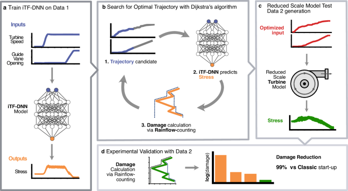
After concluding the trajectory optimization, a second campaign of measurements was carried out that included the optimized control trajectory. Across the two reduced-scale data acquisition campaigns, different sets of sensors were successfully recorded, whereas for the input parameters, the observations for both campaigns are of similar quality.

Damage computation

Damage incurred due to fatigue is estimated following standard mechanical engineering practices: The loading cycles are computed from the stress signal according to the Rainflow-counting method¹⁰. Following that, the Miner’s rule¹¹ using the Wohler curve¹⁹ quantifies the damage caused by individual load cycles and sums up their contributions to produce a single damage estimate per stress trajectory. The damage computation is carried out for each of the sensors, and the final damage estimate equals the maximum damage for the available sensors.

iTF-DNN stress model

At each time point for s sensors we observe the vector ({{{boldsymbol{y}}}}_{t}in {{mathbb{R}}}^{s}), indexed by time t = 1, …, T. For the time series of length T denote stacked vectors y_t as ({{boldsymbol{y}}}in {{mathbb{R}}}^{stimes T}): y = [ y₁, y₂, …, y_T]. The trend component of the stress is denoted by ({{boldsymbol{m}}}in {{mathbb{R}}}^{stimes T}) and the oscillatory high-frequency component is denoted by ({{boldsymbol{o}}}in {{mathbb{R}}}^{stimes T}). The control vectors are stored in ({{boldsymbol{u}}}in {{mathbb{R}}}^{qtimes T}), so that the vector ({{{boldsymbol{u}}}}_{t}in {{mathbb{R}}}^{q}) represents the control values at time t. The value of q equals 3 during model training when all inputs are used, and q = 2 during optimization, as one of the variables (the Head) is kept fixed. For multiple trajectories of observed measurements, we add additional indexing for the variables, e.g., y_j,t, t = 1, …, T_j, where j runs through the trajectory number. The stress depends on the input parameters, and we omit this dependence in the notation.

To model stresses and optimize damage, we assume that stress trends depend instantaneously on control parameters. This means that at any given time point, the values of GVO, turbine speed, and Head are sufficient to fully determine the average stress. With this in mind, we propose the following decomposition for the observed stress time series.

where m_t is a slowly varying trend, o_t is an oscillatory component, and ϵ_t is random homoscedastic noise. The stress depends on ({{{boldsymbol{u}}}}_{t}in {{mathbb{R}}}^{q}), q = 3, as additionally to GVO and turbine speed, the Head level was added due to fluctuations of the measurements from the constant value.

Our modeling choice fell on neural networks due to their ability to capture complex, nonlinear relationships in highly oscillating time series that depend on control variables. At the same time learning the high-frequency oscillations is challenging⁴²: A basic neural network model tends to learn low frequencies primarily and can struggle with approximations of high frequencies. Our work is inspired by the PFF-DNN⁴³ and PhaseDNN⁴⁴ models to improve the learning of high-frequency signals. Both models attempt to learn the signal representation in the time-frequency domain by mimicking the Short-Time Fourier Transform (STFT) of the signal (or the residual after modeling the signal trend). Note that these models aim to learn an approximation of the observed signal using neural networks with no dependence on input variables. Our case is more complex, as we are given time-varying input parameters that affect the signal dynamics and, in particular, its STFT. In what follows, we propose a model that aims to learn the dependence of the oscillatory signal dynamics on the available input control parameters. We abbreviate our model as input Time-Frequency deep neural network (iTF-DNN).

We assume m_t is deterministic and depends only on the current controls u_t, and does not depend on the previous control history. The remaining oscillatory component o_t is allowed to depend on control history in a non-instantaneous way. In particular, we estimate the amplitude and phase of the STFT of the remaining signal (after having estimated m_t) depending on the control values in the neighboring STFT windows. The estimate of the oscillatory component o_t is further recovered through an ISTFT based on the models of amplitudes and phases of the STFT. We describe the models more formally below.

For damage estimation in the case of a large spread of m_t values, the damage induced by o_t is much smaller, as according to Miner’s rule, low-frequency oscillations with large amplitudes typically have a more significant impact on cumulative fatigue damage compared to high-frequency oscillations with smaller amplitudes. Nevertheless, to obtain a general model of stresses and estimate damage precisely, it is important to model both the trend m_t and the oscillations o_t accurately.

Trend model

We model m_t by a neural network (ResNet²⁰) ({f}_{{{boldsymbol{m}}},{{{boldsymbol{theta }}}}_{{{boldsymbol{m}}}}}({{{boldsymbol{u}}}}_{t}),) where u_t are the input control parameters and θ_m are the parameters of the neural network, which are optimized by the minimization of the mean squared error (MSE) between targets y_t and the network’s predictions NN_m(u_t) on the training set of p time series of lengths T_k, k = 1, …, p until convergence:

to obtain a preliminary estimate of the trend ({f}_{{{boldsymbol{m}}},{hat{{{boldsymbol{theta }}}}}_{0}}({{boldsymbol{u}}})).

Oscillatory component

Next, we estimate the residual

between the observed stress value and the trend estimates to obtain a de-trended oscillatory signal. We model the amplitude and phase of the oscillatory residual by approximating its STFT with neural network models dependent on the controls. For simplicity of notation, assume s = 1, the extension to larger dimensions s of the output is straightforward. Consider the STFT of the residual signal (hat{{{boldsymbol{o}}}}) for one trajectory: Given a window size W and hop size S, the STFT components ({{mathcal{F}}}(hat{{{boldsymbol{o}}}})[i,l],l=1,ldots,L), L = ⌊(T − W)/S⌋, i = 1, …, ⌊W/2⌋ are calculated for L windows of length W with the hop S and a set of frequencies, indexed by i. We fixed the length of one window to W = 1024 and S = 256. For each STFT window, we get vectors of amplitudes a_l and phases ϕ_l with components

To model the amplitude and phase vectors a_l and ϕ_l, we train two vector-output ResNet neural networks ({f}_{{{boldsymbol{a}}},{{{boldsymbol{theta }}}}_{{{boldsymbol{a}}}}}) and ({f}_{{{boldsymbol{phi }}},{{{boldsymbol{theta }}}}_{{{boldsymbol{phi }}}}}). These networks take a control history ({bar{{{boldsymbol{u}}}}}_{l}), corresponding to the l-th STFT window, as input and are trained by minimizing the error in the frequency domain, combined with with the trend modeling error, using the initialization ({hat{{{boldsymbol{theta }}}}}_{0}) for the trend model parameters:

where α and λ are hyperparameters.

To obtain the estimates of o from the STFT estimate ({hat{{{mathcal{F}}}}}_{{hat{{{boldsymbol{theta }}}}}_{{{boldsymbol{o}}}}}({{boldsymbol{u}}})), ({hat{{{boldsymbol{theta }}}}}_{{{boldsymbol{o}}}}={{hat{{{boldsymbol{theta }}}}}_{{{boldsymbol{a}}}},{hat{{{boldsymbol{theta }}}}}_{{{boldsymbol{phi }}}}}), given by the models of the amplitude ({f}_{{{boldsymbol{a}}},{hat{{{boldsymbol{theta }}}}}_{{{boldsymbol{a}}}}}({bar{{{boldsymbol{u}}}}}_{l})) and phase ({f}_{{{boldsymbol{phi }}},{hat{{{boldsymbol{theta }}}}}_{{{boldsymbol{phi }}}}}({bar{{{boldsymbol{u}}}}}_{l})), l = 1, …, L, we apply an ISTFT to get ({f}_{{{boldsymbol{o}}},{hat{{{boldsymbol{theta }}}}}_{{{boldsymbol{o}}}}}({{boldsymbol{u}}},t)={{{mathcal{F}}}}^{-1}{[{hat{{{mathcal{F}}}}}_{{hat{{{boldsymbol{theta }}}}}_{{{boldsymbol{o}}}}}({{boldsymbol{u}}})]}_{t}), such that ({f}_{{{boldsymbol{o}}},{hat{{{boldsymbol{theta }}}}}_{{{boldsymbol{o}}}}}:{{mathbb{R}}}^{lfloor W/2rfloor times L}to {{mathbb{R}}}^{T}). After each optimization gradient step, the residual is estimated by (5) for the updated parameters of the trend model.

The final iTF-DNN model combines the model of the trend and the model of the oscillation

During inference, we perform forward passes through the networks to obtain trend and oscillatory predictions for a given control trajectory.

Model performance

The iTF-DNN model performance results on training and validation on the data from the first experimental campaign are shown in Table 3, namely mean and standard deviation of per-trajectory R², MSE, Bias (average of non-absolute residual values) of predictions together with (Min, Max) of observations for reference. The model has a tendency to have a small negative bias. Overall, training and validation results show good agreement between the errors on training and validation datasets.

Dijkstra optimization

Using the fitted iTF-DNN model, we implement an optimization procedure that systematically explores the space of possible trajectories to find the lowest possible damage trajectory. For the damage optimization process, we focus on the sensor exhibiting the best data quality.

Consider stresses and input control trajectories in the interval of time [0, T], sampled with the time step Δτ (at 1kHz, Δτ = 1ms). Note that the Head level was used to train the iTF-DNN, as it can fluctuate in the reduced-scale model, but during the trajectory optimization, we keep the Head fixed and optimize the damage in the Turbine Speed and the GVO. Thus, the stress depends only on two inputs: Turbine speed and GVO, that is ({{{boldsymbol{u}}}}_{t}in {{mathbb{R}}}^{q}), where q = 2.

Recall that we are trying to solve (2), the problem of finding the minimally damaging sequence of controls ({{{boldsymbol{u}}}}^{star }in {{mathcal{U}}}), where ({{mathcal{U}}}) is a space of viable trajectories, i.e., each sequence ({{{boldsymbol{u}}}}^{circ }in {{mathcal{U}}}) fulfills the constraints:

1. 1.

   Boundary Conditions: The sequence starts at a standstill and ends at operating conditions (u_op),

   $${{{boldsymbol{u}}}}_{0}^{circ }={{0}},quad {{{boldsymbol{u}}}}_{T}^{circ }={{{boldsymbol{u}}}}_{{{rm{op}}}},$$

   (11)

   where T is not limited to a specific trajectory length.

2. 2.

   Bounded increments: Neither the Turbine speed n nor the GVO g decrease at any point and the trajectory does not exceed machine limits on turbine acceleration and GVO velocity;

   $${{0}}le {{{boldsymbol{u}}}}_{t+1}^{circ }-{{{boldsymbol{u}}}}_{t}^{circ }le Delta {{boldsymbol{u}}}.$$

   (12)

3. 3.

   Allowed: The trajectory lies completely within an allowed phase space ({{mathcal{C}}}),

   $${{{boldsymbol{u}}}}_{t}^{circ }in {{mathcal{C}}}subset {{mathbb{R}}}^{2}.$$

   (13)

This problem is low-dimensional, continuous, non-convex, and bounded.

Dijkstra’s Algorithm²² is a widely used algorithm for solving the shortest path problem, i.e., the problem of finding the minimal-cost path between two nodes in a weighted graph. Starting from an initial node n₀, the algorithm iteratively considers the closest visited node (tilde{n}), and updates the distances to the nodes ({n}_{i}(tilde{n})) connected to this node. The algorithm terminates when the entire graph has been visited, or when a target node has been reached. By visiting the nodes in order of increasing cost, the algorithm is guaranteed to produce an optimal solution. Consider a discrete problem where the turbine speed and GVO take values on a regular grid, resulting in a collection of evenly-spaced nodes. To ensure the computational feasibility of the trajectory search, we consider coarsened trajectories, by effectively reducing the frequency of the data points by K. Thus, we introduce a timescale by defining the increment Δt = KΔτ. To construct the graph for the Dijkstra optimization, we set all the nodes of the grid to be its vertices: For a 2D grid defined by equidistant points along the intervals [0, u_op,1] and [0, u_op,2], with N equidistant points along each axis, the total number of points on the grid is N². Each point (x_1,i, x_2,j) on the grid can be represented as:

For each vertex, we draw edges to all nodes where a transition would not violate the bounded increments condition (12): Let n_i,j be the node at the position (x_1,i, x_2,j). An edge exists between two nodes n_i,j and n_k,l if and only if the following coordinate-wise inequality is satisfied:

Next, we compute the weights for the edges: We set the edge weights to correspond to the increase in damage incurred by extending the path from a node n^⋆ to a neighbor (tilde{n}). By setting the cost to the increase in damage, we achieve the desirable property that the cost to access (tilde{n}) is exactly the damage of the least-damaging trajectory that ends at (tilde{n}). To reconstruct the trajectory in the original time scale Δτ, for the calculation of the weight, we fill in the control values between two nodes and linearly interpolate between them at a rate of 1/Δτ.

Algorithm 1

Dijkstra-based Trajectory Optimization

Require: start_node, goal_node, priority_queue, cost, parent, visited

1: While priority_queue is not empty do

2:  (current_cost, current_node)  ← heappop(priority_queue)

3:  if current_node == goal_node then

4:   break

5:  end if

6:  for neighbor in get_neighbors(current_node) do

7:   path  ← reconstruct_path(parent, current_node) + neighbor

8:   trajectory  ← interpolate_trajectory(path)

9:   stress  ← calculate_stress(trajectory)

10:  new_cost  ← compute_damage(stress)

11:   if neighbor not in cost or new_cost  < cost[neighbor] then

12:    cost[neighbor]  ← new_cost

13:    parent[neighbor]  ← current_node

14:    heappush(priority_queue, (new_cost, neighbor))

15:   end if

16:  end for

17: end while

18: optimal_path  ← reconstruct_path(parent, goal_node)

19: return optimal_path, cost[goal_node]

The described graph is used for the trajectory optimization problem (2) with the help of Dijkstra’s Algorithm 1 with the starting node set to (0, 0) and the end and limit nodes u_op = (736, 17). Note that the maximum start-up duration, ({T}_{max }), is related to N and K by (2Ncdot (K{{rm{ms}}})={T}_{max }) and that the number of edges that need to be explored per node is of the order E_node ∝ K²N² due to (15). The total computational complexity of the algorithm is dominated by the number of edges E_nodeN^{2 45}. Combining these observations, the complexity scales as E_nodeN² ∝ N². We have selected the time resolution K = 128 and the number of points N = 256, by manual adjustment as a compromise between the computational complexity and the time discretisation step of the optimized trajectory, given a maximum start-up duration ({T}_{max }=65{{rm{s}}}).

To ensure viable trajectories are produced, we impose a limit on turbine acceleration and GVO angular velocity (12), corresponding to machine limits, which are 280rpms⁻¹ and 2.16^∘s⁻¹ correspondingly. Additionally, we disallow parts of the phase space (13) since they would require active braking of the turbine to traverse or contain regions where the trend iTF-DNN is particularly uncertain about its prediction. See Fig. 4a for the disallowed region.

Equivalent time at Best Efficiency point quantification

At best efficiency point (BEP) the turbine converts the specific hydraulic energy and the angular momentum of the flow into mechanical energy with minimal losses, thus reaching the BEP. This depends on the hydraulic machine geometry and control parameters of the operating condition. The equivalent time at BEP expresses the operational time of a hydraulic turbine as if it had been running continuously at its ideal conditions (BEP)¹⁶. To quantify the equivalent time at BEP, we rely on steady-state stress measurement collected during the second campaign. By analyzing a 20-second stress measurement collected at the BEP, we calculate the damage incurred per second. We divide the damage incurred during one start-up by this value to derive the equivalent time at BEP. Note that in this study the term BEP trajectory is reserved for a start-up sequence, tracking the BEP for each rotational speed during the machine acceleration from 0 to nominal rotational speed.