GODEEEP-hydro: Historical and projected power system ready hydropower data for the United States

Meteorology Data

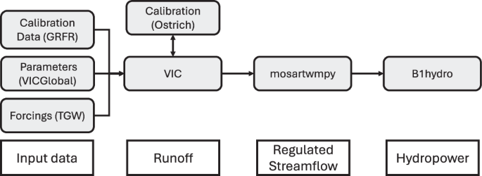
In this study we used perturbed thermodynamics experiments^3,4 (https://tgw-data.msdlive.org/) as meteorological forcing. The forcing data is a 1/8th degree dynamically downscaled product which contains both historical data and future projections over the contiguous United States (i.e. lower 48 states), southern Canada, and northern Mexico. The dynamically downscaled data is produced by initializing a WRF⁵ model using ERA5⁶ boundary conditions. The future projections are developed by replicating the historical period (1980–2019) twice in the future (2020–2059, 2060–2099) while applying a warming signal that is derived from groups of Coupled Model Intercomparison Project (CMIP) 6 models.⁴ The warming scenarios are labeled as rcp45cooler, rcp45hotter, rcp85cooler, and rcp85hotter which represent a range of warming signals derived from climate models using the representative concentration pathway (RCP) 4.5 and 8.5 emissions scenarios.

Hydrology Model

For hydrologic modeling we use the variable infiltration capacity (VIC) model^7,8 (https://vic.readthedocs.io/en/master/). VIC is a commonly used model for large scale distributed hydrologic modeling studies. Parameters are obtained from the VICGlobal⁹ dataset which contains vegetation and soil parameters on a 1/16th degree grid. We calibrate the parameters against the Global Reach-level River Flood Reanalysis data¹⁰ which is a global dataset of 1/20th degree runoff. Calibration is conducted for 1981–2000 at 1/16th degree resolution on a grid cell by grid cell basis. For automatic calibration we use the dynamically dimensioned search (DDS) algorithm¹¹ through the Optimization Software Toolkit for Research Involving Computational Heuristics (OSTRICH) framework¹² (https://doi-bor.github.io/ostrich/). The DDS algorithm is designed to provide a reasonably optimal solution within a limited computational budget, here we used 100 iterations of the DDS algorithm as testing indicated that more iterations provided marginal improvement to the objective function value. For the objective function we used the Kling-Gupta Efficiency (KGE) metric of monthly observed runoff as it provides a good balance between low and high runoff conditions. The KGE metric is described further in the validation section. Table 1 shows the calibration parameters and the ranges which are selected based on previous hydrologic studies using the VIC model^9,10,13,14.

Routing and Water Management Model

Routing is conducted at a 1/8th degree scale by the mosartwmpy model¹⁵ (https://mosartwmpy.readthedocs.io/en/latest/), a Python implementation of the MOSART-WM model,^16,17 which is part of the Energy Exascale Earth System Model (E3SM) (https://e3sm.org/). Routing alone produces gridded natural streamflow estimates but water management is required to develop estimates of regulated streamflow, storage, inflow, and outflow for hydropower projects, which mosartwmpy produces through the use of data driven reservoir operation rules¹⁸. Hydropower projects were mapped to the 1/8th degree grid as part of the 9505 federal assessment of hydropower¹⁹.

Hydropower Model

The final model in the chain takes the regulated streamflow values produced by mosartwmpy and generates weekly and monthly hydropower estimates, which we call B1hydro. At every hydropower plant, B1hydro models the power generation as a linear regression model with the form:

where P_t is the power at time t, O denotes the outflow, I denotes the inflow, S denotes the storage, which are outputs from the mosartwmpy model, β_i,j are the regression parameters, and ε_t is the normally distributed error term. The lag parameter n is set to 12 and 52 for the monthly and weekly model respectively to account for annual hydrologic variability.

The data used to calibrate the regression parameters is the HydroWIRES B1 data^20,21 (https://github.com/HydroWIRES-PNNL/B1-data), which contains weekly and monthly hydropower estimates that are disaggregated from U.S. Energy Information Administration (EIA) annual data²². The data is available for 2001–2019 which is used as the calibration period to develop both the historical and future hydropower data at every available hydropower plant location. Of the 1492 plants in the HydroWIRES B1 data, 1452 are included in the GODEEEP-hydro dataset, with the 40 plants excluded due to records that were too short (less than 2 years) or containing all zero values (i.e. decommissioned). The entire historical period (1982–2019) is included in the final dataset to provide (1) validation with observations and other derived datasets, (2) an extension the historical record beyond what is available in the HydroWIRES B1 data, and (3) a consistent record of hydropower that is coincident with other datasets derived from the perturbed thermodynamics experiment data (e.g.²³).

In addition to total generation over the weekly or monthly period, the B1hydro model provides minimum and maximum power generation of the period and the average daily operational range (ador), which are directly useful in power system models. These values are defined as:

where P_max,t and P_min,t are the max and min allowed power generation at time t, P_ador,t is average daily operational range at time t, P_t is the average power generation at time t, P_np is the nameplate capacity of the plant, and a_max, a_min, and a_ador are parameters with values between 0 and 1 which can be derived from hourly power generation data.

Hourly hydropower generation is usually proprietary and business sensitive and therefore not publicly available. The Army Corps of Engineers Northwestern Division, which includes the Columbia River Basin, is one exception where historical hourly generation data from most federally-operated hydropower facilities is published on the Dataquery platform (https://www.nwd-wc.usace.army.mil/dd/common/dataquery/www/). The B1hydro model uses this hourly generation data to estimate the min and max power and ador at every hydropower plant in this study by assuming that a_max, a_min, and a_ador are equal to the average parameter values from all the hydropower facilities on the Dataquery platform. This approximation allows for reasonable constraints to be developed for power system models given the scarcity of publicly available hourly hydropower data.

Future Simulations

The four future climate scenarios in the TGW data (rcp45cooler, rcp45hotter, rcp85cooler, and rcp85hotter) are used to develop future hydropower simulations from 2020–2099. The calibrated VIC model is used to produce future runoff simulations for each scenario, which are then run through mosartwmpy, and finally the calibrated B1hydro model is used to produce monthly and weekly hydropower generation estimates.